The Problem

Type II diabetes is one of the most prevalent conditions in the world, affecting over 400 million people worldwide. Left untreated, type II diabetes could cause serious, life-threatening complications including: heart disease, stroke, and blindness. Some of the main factors that lead to the development of type II diabetes are lifestyle related. Lack of exercise as well as improper diet can lead to onset of diabetes. Furthermore, genetics seems to play a major role as well. Prevalence of diabetes in close familial relatives leads to increased chances of developing the condition as well. Lastly, multiple bouts of gestational diabetes, a diabetic condition that occurs during pregnancy, can lead to chronic type II diabetes well after childbirth.

Because the correct diagnosis of diabetes is extremely vital, I decided to predict the diagnosis of type II diabetes using a Classification Algorithm. I then made a Flask web app to share my predictive power with the world!

The Data

Studying a random population for diabetes poses many challenges, mainly due to unquantifiable genetic variation within any population. Because genetics plays a pivotal role in the chances for type II diabetes affliction, not understanding or knowing this aspect in the study group would lead to an improper and most likely incorrect model.

Luckily, Kaggle posted a dataset about various physiological features taken fro females over the age of 21 from the Pima Indian population of Arizona. The Pima Indians, a Native American population, pose a unique opportunity for diabetes researchers due to their limited European admixture. This posits the greatest opportunity to study diabetes with the uncontrollable genetic factor playing the smallest possible role.

The features of the dataset:

Age: age of patient

BMI: body mass index (weight in kg/(height in m)^2)

Skin Thickness: triceps skin fold thickness (mm)

Blood Pressure: diastolic blood pressure (mm Hg)

Diabetes Pedigree Function: 0:1 value generated from familial diabetes history/risk

Pregnancies: number of times pregnant

Glucose: concentration of glucose in blood 2 hrs after ingestion of sugary drink (mmol/L)

Insulin: concentration of insulin in blood 2 hrs after ingestion of sugary drink (μU/mL)

Modeling

First Pass

Before starting my modeling, I needed to decide on which classification algorithm to use. Because my problem involves the diagnosis of a potentially lethal medical condition, I chose algorithms with the utmost interpretability.

KNN k-nearest neighbors: Class is chosen based on class of k nearest data points based on euclidean distance

Logistic Regression: Class is chosen based on highest probability of being either a 0 or 1 (more on this later).

Naive Bayes: Algorithm assumes independence of all events. Chooses class based on highest probability of observing the data based on class.

Random Forest: An ensemble decision tree method that constructs numerous decision trees based on sampling with replacement of the original dataset. In addition, each split of the tree based on a random subset of features. This deals with decion tree’s common problem of overfitting.

After performing a test/train split, I trained each of the above models with my data. I then get testing accuracy using a stratified (class balance is maintained) k-fold split (10 fold). The following graph shows my results:

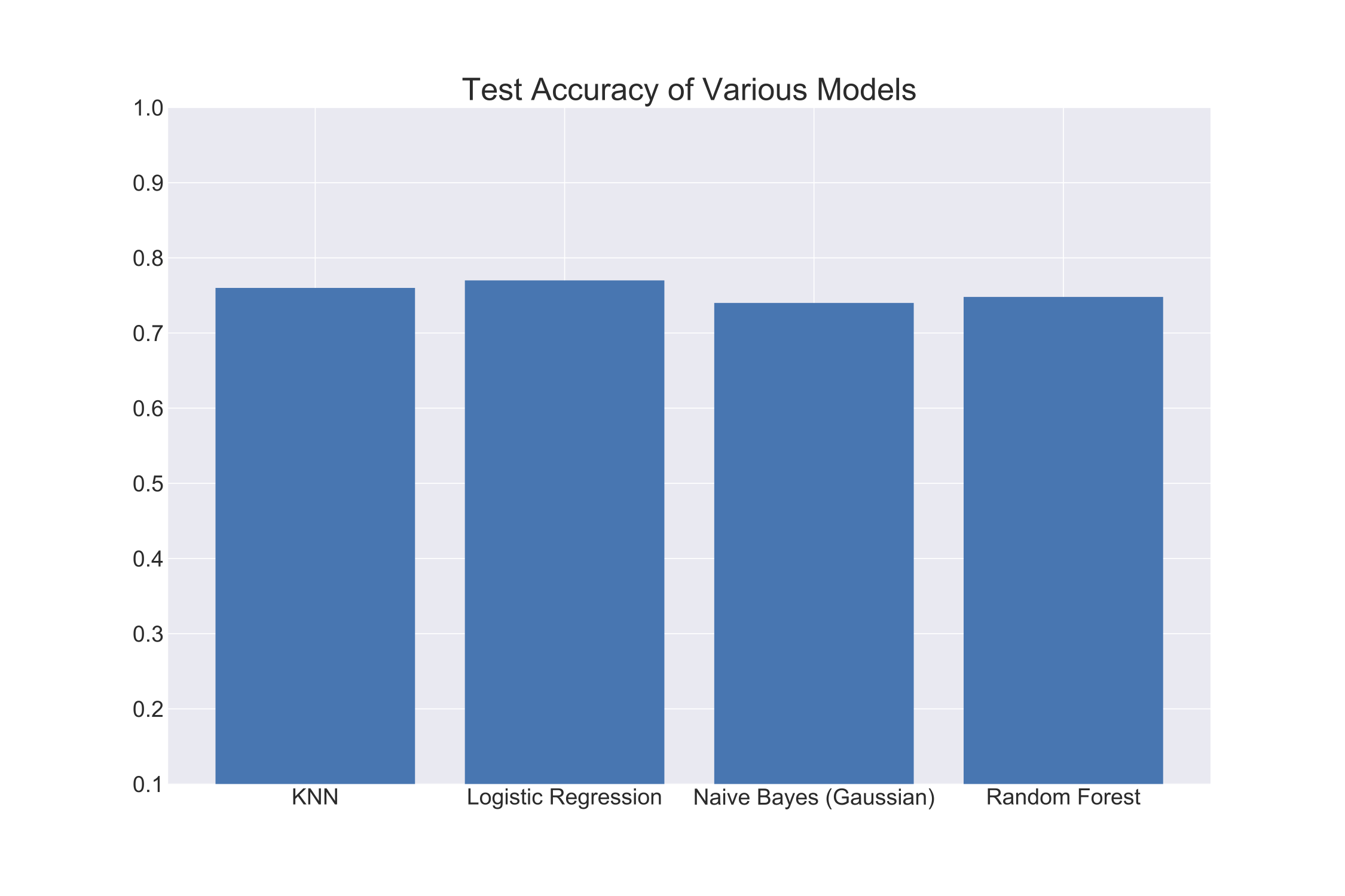
As you can see, Logistic Regression performed the best with an accuracy of about 78%. Yet, all the other algorithms performed similarly well. I chose to go with Logistic Regression as my classification algorithm for its clear interpretability and its superior performance.

First Logistic Regression Model

As a first pass at modeling, I decided to include all of the features listed above to run a Logistic Regression model. After performing a 10-fold stratified cross validation, my model was able to achieve an accuracy of 79%. However, this number only gives part of the story, I also needed to look at the metrics of precision (true positives/true positives+false positives) and recall(true positives/true positives+false negatives).

For my first model, I achieved the following metrics:

	Precision	Recall
Healthy	81%	91%
Diabates	73%	54%

With a recall of only 54% for the positive diabetic class, I needed to do better. Because diabetes is a potentially deadly disease, I didn’t want to run the risk of misclassifying an actual diabetic as non-diabetic. To account for this, I needed to adjust the classification threshold.

As I mentioned before, the Logistic Regression essentially outputs probabilities that a data point is either a 0 (negative) or 1 (positive). Based on a threshold, it will assign class labels. The default parameter in the sklearn logistic regression is a threshold of 0.5 (higher probability for 1 than 0.5 leads it to be classified as a 1). How will, I decide what the optimal threshold for my model is? I will use a precision recall curve.

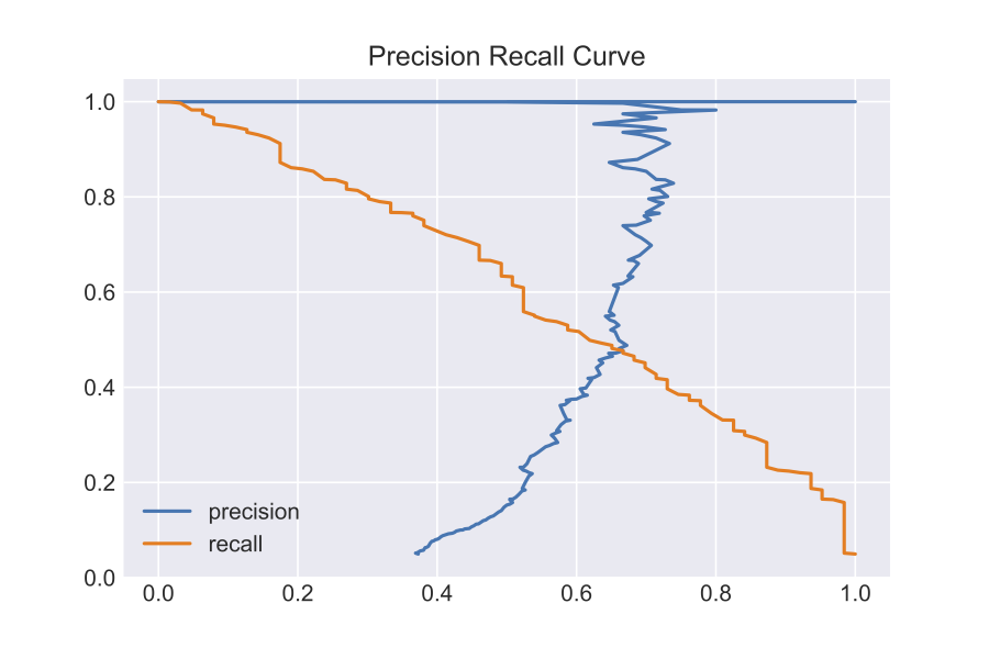
Based on looking at the curve, I will set my optimal threshold as 0.35. With this new threshold, I achieved the following metrics:

Test Accuracy: 82%

	Precision	Recall
Healthy	90%	82%
Diabates	67%	80%

Although I had to sacrifice some precision, I was able to achieve a much higher recall of 80%. I was willing to sacrifice some precision because those improperly classified as diabetic might be hovering on the cusp of pre-diabetes and should probably seek medical attention.

With my improved model, I got the following key features for predicting a diabetes diagnosis:

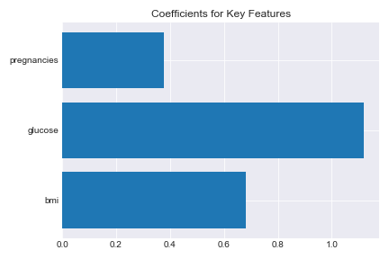
Glucose concentration, bmi, and number of pregnancies were the strongest features for classifying a positive diabetes diagnosis. But what do these coefficients really mean?

Interpreting a Logistic Regression Model

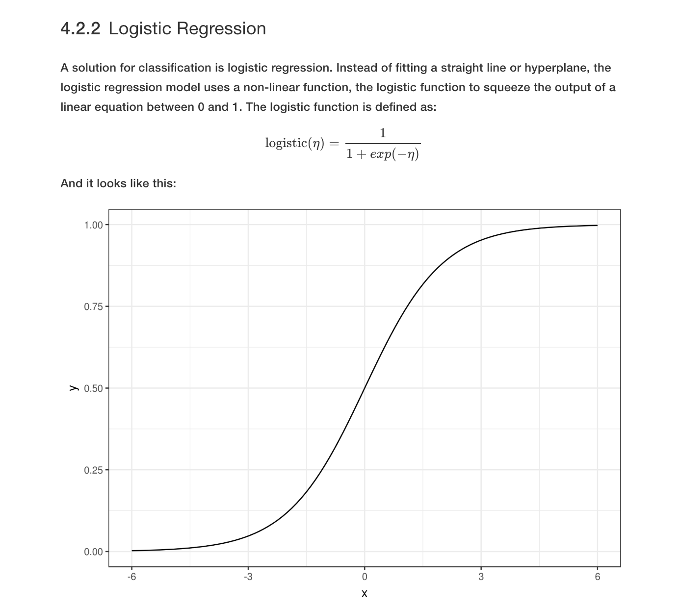
The following figure explains the concept of the logistic function. Essentially, the linear model which can range from -∞ to ∞ is squished to output only from 0 to 1 (this value represents the probability of being a positive, 1 class).

Resource for Interpreting Machine Learning Models

Since the linear function is wrapped in the logistic function (output from 0 to 1), we can’t interpret the results of the regression linearly. So, we need to transform the linear function into something more interpretable. To do this, we will use the log odds:

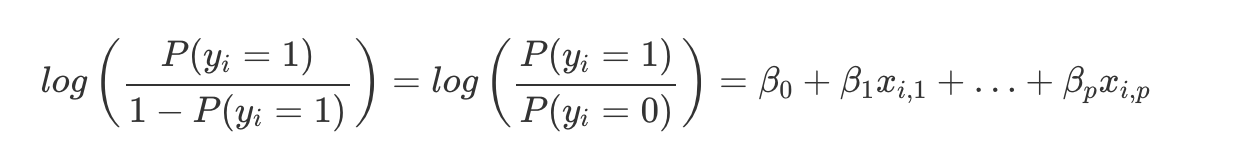
The inner term represents the odds ratio of classifying as a 1 or 0. Odds are essentially the probability of a 1 divided by the probability of a 0.

Taking the log and rearranging allows us to interpret the coefficients of the logistic regression.

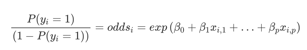
Basically, what this means is that a unit increase in a feature x, can be interpreted as an increase in the odds ratio of classifying as a 1 by a factor of e^(coefficient weight).

This can be complicated but to give a simple example, in my above model, the coefficient weight for bmi was about 0.7. This means, for every standard unit increase in bmi, the odds ratio for being classified as diabetic is multiplied by a factor of e^(0.7) or about 2.01.

So, if the odds ratio was initially 2, an increase of one standard unit of bmi would change the odds ratio to 4. That’s it!

Simpler Logistic Model

Now that we have an understanding of Logistic coefficients, I wanted to share another Logistic Regression model I made with the dataset. I wanted to make a model that was extremely simple. This means, I wanted to make a meaningful model that could be used with only the simplest of features, features that any person could reasonably surmise within 30 mins or so. I also wanted to make sure people that have never been or aren’t capable of being pregnant to gain insight from my model.

So, in order to keep with this idea, I decided to eliminate the following features from my model: glucose, insulin, diabetes pedigree function, pregnancies, and skin fold thickness.

This left me with only the features of age, bmi, and blood pressure.

After fitting the Logistic Regression model, I achieved the following metrics:

Test Accuracy: 63%

	Precision	Recall
Healthy	77%	61%
Diabates	48%	66%

The coefficients for the model:

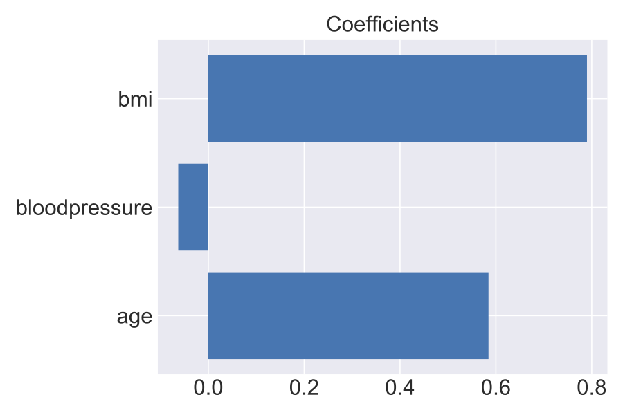
As expected, bmi and age play a significant role in determining if a person would be classified as diabetic in absence of all the other features. In fact, the Mayo Clnic lists these three factors as key indicators of Type II diabetes risk.

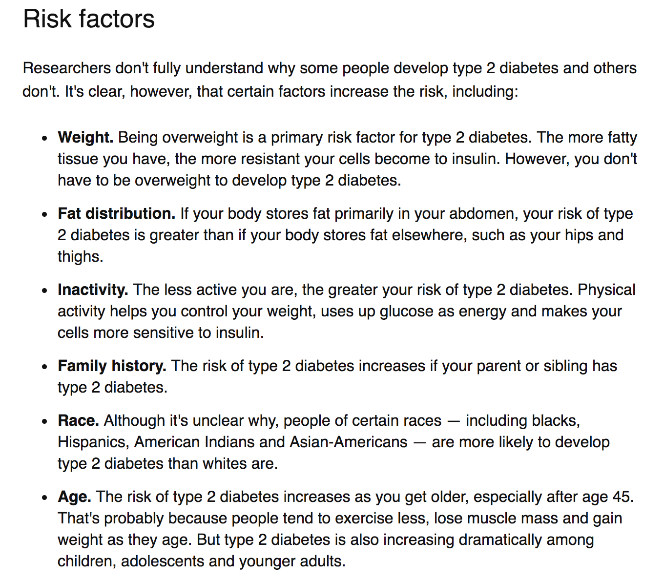
Although this model didn’t perform as well as one would hope, it highlights one of the key deficiencies of a diabetes diagnosis. Even if you are aware of the risk factors actual medical doctors recommend being wary of (age, bmi, blood pressure), the model was only 63% accurate. This is only 13% better than random guessing (assume everyone is diabetic). So, I beleive the key takeaway from this project is that if you even slightly suspect you may be at risk for diabetes, you should see a doctor immediately! Even knowing the risk factors seems to be a flip of the coin!

In order to try out the Flask App I made, please use the following link:

Diabetes Predictor App